Earl: a framework for scalable reinforcement learning research
In this post I will briefly describe Earl, a reinforcement learning (RL) framework I wrote that enables scalable distributed training across multiple devices, and discuss some of the things I learned along the way.
Earl implements the two architectures described in “Podracer architectures for scalable Reinforcement Learning”, which were used at DeepMind to scale training to very large batch sizes across many chips. Note these are not neural network architectures, but distributed RL architectures that can be used to train models that internally may use any neural network architecture. To prove it is usable, I used Earl to implement the R2D2 algorithm as described in another DeepMind paper “Recurrent Experience Replay In Distributed Reinforcement Learning”.
Background
To provide context, I’ll briefly summarize the Podracer architectures paper. If you know it, feel free to skip this.
In contrast to other machine learning paradigms, online RL involves an agent and an environment, and the training data is generated on the fly from their interactions. The paper describes two architectures: Anakin and Sebulba1. Anakin is used when an environment is compatible with jax.jit, and Sebulba is used otherwise. In both of the architectures, the agent is implemented in JAX and is compatible with jax.jit. If you’re not familiar with JAX, see my introduction. Basically, code that is run under jax.jit is optimized by a compiler and run on any supported device (e.g. GPU) without further involving the Python interpreter.
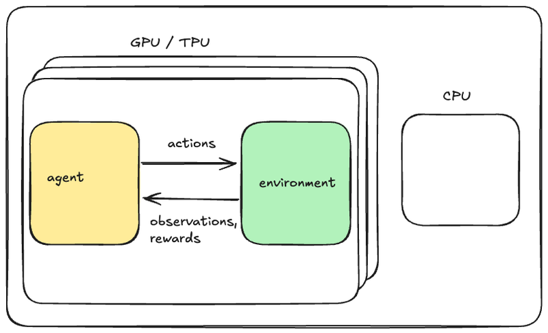
In Anakin, one can have the entire training loop (agent + environment interaction, loss function and optimization) happen under jax.jit and thus run on a device (e.g. GPU) without going back to the Python interpreter. In terms of writing a performant training loop, in some ways this is even easier to deal with than normal (supervised) machine learning since one does not need to copy any data from the host to the accelerator. Scaling this across multiple devices is trivial using JAX.
Below is a figure I created that is analogous to the paper’s figure 3 (see below) that illustrates Anakin-style RL. Notice that there is nothing running on the CPU! This figure may be misleading because the arrows don’t necessarily signify data being copied. It’s just data that is produced by one function being an argument to another function.
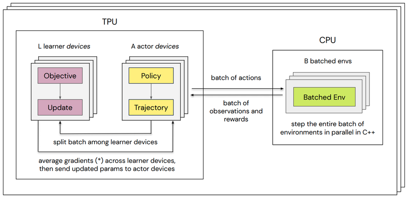
Although jax.jit-compatible environments are gaining more adoption in research, there are still many environments that can’t run under jax.jit that researchers care about. The Podracer solution to training on these at scale is called Sebulba. Sebulba involves splitting agents into actor and learner as shown in Figure 3 from the paper. Note that in this figure the arrows do signify data copies.
One of my main goals with Earl was to have a single agent implementation that could easily be run in either architecture. This is in contrast to what the team behind the Podracers paper did; the paper suggests they implemented agents twice, once for Anakin and once for Sebulba.
The “pod” in “Podracers” is an allusion to a collection of TPUs that are all connected with high bandwidth. Later in this post I will discuss what advantages TPUs actually provide.
Gymnax Loop: Earl’s Anakin
Earl’s implementation of Anakin is GymnaxLoop. Gymnax is a collection of RL environments implemented in JAX with a common interface, and Earl adopted that interface because it seemed more widely used than the alternatives. The GymnaxLoop implementation is mostly straight-forward, so here I only discuss some of the trickier things that I solved.
Avoiding recompilation
The first time a jax.jit function is run, it is compiled, which is slow. Unwanted recompilations are a performance foot-gun, so by default Earl will fail if the code is recompiled. When I enabled this failure, I learned that my Gymnax Loop was recompiling the main loop (act and learn) because the types of some part of the environment state were changing. After digging into it (made difficult due to a JAX bug that I reported) I discovered that the change was that the initial state (returned by env.reset()) had weak_type=True on some arrays, but calls to env.step() changed the weak_type to False. GymnaxLoop fixes this by setting weak_type=False on all arrays in the environment state before running. This avoids recompilation and thus speeds up training significantly.
Gymnasium Loop: Earl’s Sebulba
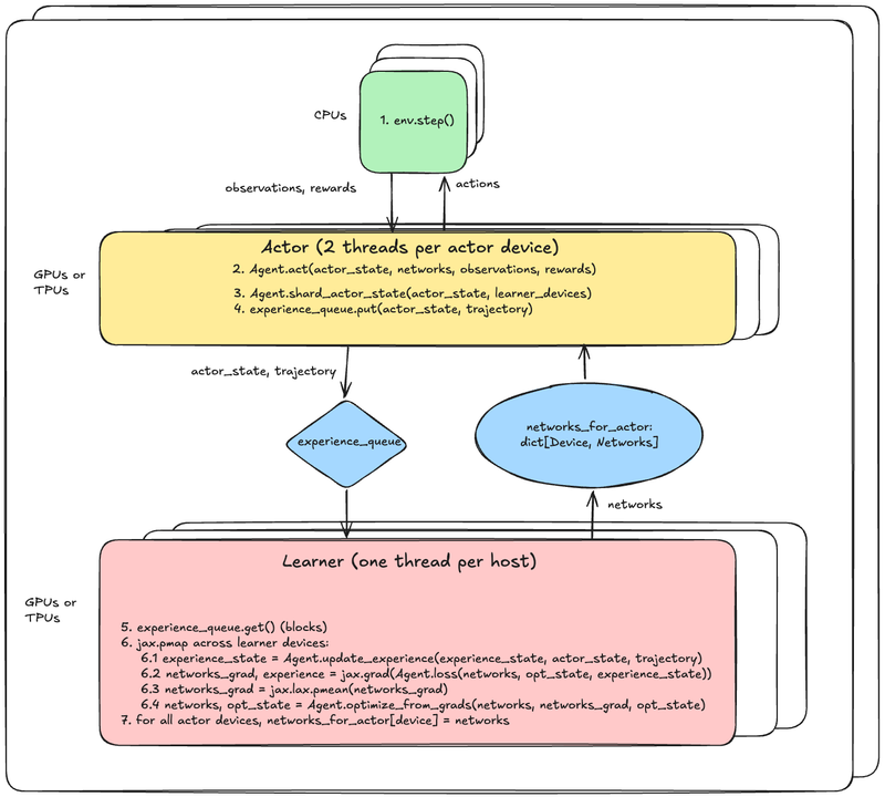
Earl’s implementation of Sebulba is GymnasiumLoop. Gymnasium is a widely-used interface for RL environments, which generally are not compatible with jax.jit. The GymnasiumLoop has a much more complex design, was much trickier to implement correctly and was also harder to optimize for performance.
Here’s a diagram showing the system architecture. Sorry the text is a little small. You can open the image in a new window to zoom in.
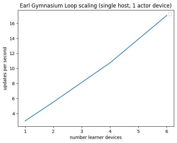
And here are results from a test showing linear scaling on up to 6 learner devices (TPU v2 cores):
Before going further into details, why is all this complexity needed in the first place? That is never explicitly addressed in the podracers paper. I think the key thing is that in a naive loop of env.step(), agent.act(), the device (GPU) will be idle during env.step() and the CPU will be idle during agent.act(). So we can get much better throughput by double buffering: have one batch of actions being computed by the agent at the same time that a batch of observations is being computed by the environment. But in order to take advantage of this double buffering, you need the learning to be able to learn from batches of trajectories from different sets of environments that are delivered out of order. And that basically implies an actor-learner split, and once you’ve split the agent thus, one can get further throughput gains by scaling the number of actors and learners independently. And that’s basically the architecture: separate sets of actors and learners, communicating asynchronously, scaled independently.
OK, now some details.
Agent state organization
A key design challenge was creating a flexible agent architecture that could work efficiently in both Anakin and Sebulba paradigms. Earl has two main base classes: AgentState and Agent. These are structured to enable Sebulba-style training while attempting to leave the user lots of freedom (they’re also used for Anakin-style training but they’re way too complex if that’s the only thing you need).
AgentState has the following fields:
- Actor. This is read and written by the actor. This is also read by the learner when calculating the loss. In agents that use recurrent networks, this includes the recurrent hidden states.
- Nets. This holds the neural networks This is read by the actor. It is read and written by the learner. Anything that needs a gradient computed needs to be in the networks.
- Opt. Anything other than nets that also needs to be updated when optimizing (i.e. updating the networks). This is where optimizer state belongs.
- Experience. This is state that is based on the trajectories accumulated by actors and sent to the learners. For agents that use experience replay, this contains replay buffers.
And the key methods in Agent are:
act(self, actor_state: _ActorState, nets: _Networks, env_step: EnvStep) -> ActionAndState[_ActorState]update_experience(self, experience_state: _ExperienceState, actor_state_pre: _ActorState, actor_state_post: _ActorState, trajectory: EnvStep) -> _ExperienceStatepartition_for_grad(self, nets: _Networks) -> tuple[_Networks, _Networks]loss(self, nets: _Networks, opt_state: _OptState, experience_state: _ExperienceState) -> tuple[Scalar, _ExperienceState]optimize_from_grads(self, nets: _Networks, opt_state: _OptState, nets_grads: PyTree) -> tuple[_Networks, _OptState]shard_actor_state(self, actor_state: _ActorState, learner_devices: Sequence[jax.Device]) -> _ActorState
The method signatures and AgentState structure force algorithms to be implemented such that GymnasiumLoop can run any agent in a scalable manner.
Implicit double buffering
When I first thought about double buffering I thought I would write code that used two CUDA streams to overlap work. I was surprised to learn that JAX does not expose CUDA streams or any similar abstraction. Upon re-reading the Podracers paper, I noticed they wrote:
To make efficient use of the actor cores, it is essential that while a Python thread is stepping a batch of environments, the corresponding TPU core is not idle. This is achieved by creating multiple Python threads per actor core, each with its own batched environment. The threads alternate in using the same actor core, without manual synchronization.
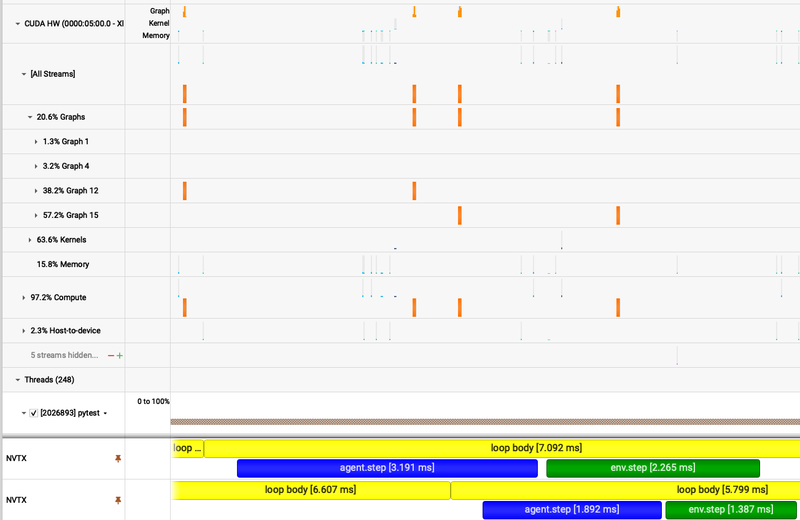
So I tried just having multiple threads use the same device, and lo-and-behold I got a huge speedup! Looking at a profile in Nvidia Nsight Systems revealed that under the hood, JAX had analyzed the computations coming in from the different threads, determined they were independent, and scheduled them on separate CUDA streams (really separate CUDA graphs). This is in contrast to PyTorch which by default puts all work on a single stream and requires the user to specify another stream if desired.
Below you can see the Nsight Systems UI showing the different CUDA graphs at the top and the agent.step() overlapping with the env.step() at the bottom. The two graphs of interest are 12 and 15. The profile records which thread launched each graph which confirmed that the two threads were launching separate graphs.
Batching and sharding data
The paper suggests that experience data is copied from the actors to the learners one batch at a time. This seems quite inefficient. I instead break up acting into cycles of configurable length, and copy one cycle’s worth of batches at a time from the actor to the learners (i.e. num_envs * steps_per_cycle units of observations, actions, rewards, etc).
The paper does not address the details of how the data is stored and retrieved for replay. In Earl, the user specifies num_envs, which for GymnasiumLoop is the number of environments per actor thread. There are two actor threads per actor device. Each actor thread shards the trajectory and actor state evenly across the learner devices. Thus when the framework calls Agent.update_experience() on the learner device, the experience data has batch size = num_envs / len(learner_devices), which must be an integer (i.e. must divide evenly). The Agent is free to store and replay that experience in whatever way it chooses. For my R2D2 implementation, to keep things simple, I store the experience using that same batch size (num_envs / len(learner_devices)) and then replay some batch size that is an integer multiple of that batch size.
One thing not mentioned in the paper but which is obviously necessary for many algorithms is copying of actor state to the learners. For example, in R2D2 the LSTM hidden states at the beginning of a trajectory are needed by the learners. The framework can take care of properly distributing the observations, actions and rewards, but the details of the actor state depend on the particular agent implementation, so users of GymnasiumLoop have to implement Agent.shard_actor_state(actor_state, learner_devices). Depending on the algorithm, some elements of the state will be sharded evenly to go along with the trajectory data, while other elements will be replicated across all learner devices or not copied at all.
Performance tuning
In GymnasiumLoop, ideally all accelerator devices are being fully utilized. Getting there requires a lot of tuning. Some of the knobs available for tuning and what they do:
- Num_envs: the number or environments per actor thread (there are 2 actor threads per actor device). Increasing this will increase CPU usage during env.step() and increase actor device (e.g. GPU) usage during agent.act(). It will increase CPU memory usage (for the environment state). It will also increase memory usage on the actor device, moreso if the actor maintains per-environment state (e.g. recurrent hidden state).
- Num_off_policy_optims_per_cycle: the number of times Agent.loss and Agent.optimize_from_grads is called between waiting for new experience data from the actors. Increasing this will increase learner device usage. It may cause the actor threads to block (and thus make the actor devices and CPUs idle) if the queue for experience data is full (currently the queue has a max length of 2). Increasing it will also make the algorithm more off-policy, since it does more updates on experience that was produced by older policies.
- The number of actor devices and learner devices. More learner devices effectively increases batch sizes and thus can help training be faster or more stable. More actor devices increases the rate at which new experience trajectories are made available to the learners. If the number of environments on a machine is limited by CPU cores or CPU memory, increasing the number of actor devices effectively reduces the actor batch size (num_envs).
The metrics that are currently exposed on every run are the cycle time for the learners (which includes getting new experience and then some number of loss + optimization steps), and the time the learners spend waiting for an actor to enqueue experience. Because JAX arrays are materialized asynchronously, the actor thread’s call to jax.device_put_sharded() will return before the data has actually been copied to the learner devices. Thus the learner device will be able to successfully retrieve experience from the queue, but computation may block waiting for the data to be copied. I don’t think there’s a good way to expose the exact amount of time spent waiting for copies during normal execution (doing so would require putting in barriers that could hurt performance). So the process I used for tuning performance was:
- If learner device utilization is not high, try tweaking the above knobs to get it up.
- When / if that didn’t succeed, use a profiler (I used NVidia Nsight Systems). This made it fairly easy to see when computation was waiting on copies.
Performance footgun: implicit vs explicit host->device copies
Using the profiler I was able to spot a blocking host->device copy in the inner loop of the actor cycle that was caused by something like:
for _ in steps_per_cycle:
  observation, done, reward = env.step(action)
  observation, done, reward = jax.numpy.array(observation), jax.numpy.array(done), jax.numpy.array(reward)
  action = agent.act(observation, done, reward)
It turned out that the explicit conversion from Numpy to JAX arrays was much much slower than just passing the Numpy arrays directly into Agent.act. I confirmed the issue with this simplified example:
import numpy as np
import jax

@jax.jit
def add(a, b):
 return a+b+1

def lazy():
 a = np.ones((128, 128))
 b = np.ones((128, 128)) * 2
 return add(a, b)

def eager():
 a = jax.numpy.array(np.ones((128, 128)))
 b = jax.numpy.array(np.ones((128, 128)) * 2)
 return add(a, b)
The lazy function takes 0.3 milliseconds and the eager takes 1.1 (3.7x slowdown) on a Google Colab instance with a T4 GPU.
Under the hood, the eager function launches 3 CUDA kernels, one for each array copy and one for the addition, returning to the Python interpreter between each. The lazy function goes into CUDA only once.
Batching Gymnasium environments
In the podracers paper section in Sebulba they write: To minimise the effect of Python’s GIL, when stepping a batch of environments in parallel, each Python actor-thread interacts with a special batched environment; this is exposed to Python as a single environment that takes a batch of actions and returns a batch of observations; behind the scenes it steps each environment in the batch in parallel using a shared pool of C++ threads.
The functionality described in the paper is provided for some environments by EnvPool. For Gymnasium environments not supported by EnvPool, Earl will apply Gymnasium’s built-in vectorization which uses Python multiprocessing to run multiple copies of the environment in parallel. This is much much slower than EnvPool, and one fun thing I had to work around was that each subprocess would try to pre-allocate most of the GPU memory on startup (this happens whenever you import jax). I worked around this by setting an environment variable telling JAX to only use the CPU in those environment subprocesses.
Potential improvements
Pmap -> automatic parallelism
When the Podracers paper was written, jax.pmap was the recommended way of parallelizing computation across multiple devices. Since then, the JAX team has developed “automatic parallelism” and encourages its use over pmap. The basic idea is that the programmer shards (or replicates, which in JAX is called a type of sharding) arrays across devices, and the compiler and runtime automatically figure out where computation should happen and where function outputs should go.
I prototyped an implementation of GymnaxLoop that used automatic parallelism before throwing it away and settling on the explicit Pmap approach. The reason is that I couldn’t convince myself that sampling randomly from a replay buffer wouldn’t result in extra cross-device copies and uneven workloads. Earl is currently entirely agnostic to how an agent manages its experience state (which will include the replay buffers). Experience replay could be implemented in a way that is compatible with automatic parallelism (I believe the main constraint is that buffer has to be sized such that it can be sharded evenly across devices, and reads and writes are balanced across all devices), but guaranteeing this would require the framework to be more opinionated about how replay buffers are managed.
If I were to do this, I would look to DeepMind’s Acme for inspiration. It is extremely prescriptive about how experience state is managed, and I think a similar design could result in something that’s guaranteed to be performant with JAX’s automatic parallelism.
Multiple losses
Some algorithms compute different loss terms for different subsystems. Earl doesn’t currently support this, but it wouldn’t be too hard to add.
Scaling to multiple machines, or how special are the “pods” really?
Earl currently only supports single-machine training. Supporting multi-machine would be as straightforward as adding a call to jax.distributed.initialize() in the training script. However, when scaling to multiple machines, network bandwidth becomes a critical factor. Let’s analyze how bandwidth affects training throughput and compare TPU pods with modern GPU clusters.
The “pod” in the “Podracers” article is a reference to a Google Cloud TPU pod, which is a group of TPU chips that have high bandwidth interconnections. Let’s analyze how bandwidth affects training throughput. Both Anakin and Sebulba have to send gradients between all learner devices before every optimizer step, and this latency cannot easily be hidden by overlapping that work with other work (unlike the transfers from actors to learners, which can be overlapped with both acting and learning). The amount of data that needs to be meaned is: (bits per gradient) x (num parameters).
Let’s say each device has bandwidth of R bits / sec and the gradients take S bits. Assuming the mean is calculated and sent back using a reduce-scatter and then all-gather, the time taken is:
Now let’s try to get some sensible values of R and S. Most online RL research uses relatively few parameters compared to modern LLMs (e.g. Dreamer v3 XL has 300 million parameters, the unusually large Gato has 1.2 billion). To work an example, let’s say we use 16 bits per gradient x 1 billion parameters = 16 Gbits. The TPU v6e has R = 3584 Gbps of inter-chip interconnect bandwidth, which gets us:
To answer how special TPU pods are, let’s compare this to NVidia GPUs. NVidia’s GB200 can connect up to 72 GPUs at 1800 Gbps. The same reduction would take
Roughly twice as long, but in order to determine how much of an impact this makes on training throughput we’d need to look at a particular example which depends heavily on hyperparameters. It seems the TPU networking is still higher bandwidth, but for workloads that fit within an NVLink switch, the impact on training throughput may be quite small.
Conclusion
Years ago only DeepMind and OpenAI could do distributed RL at scale. Today, thanks to the libraries, APIs, on-demand cloud computing, and knowledge that is available, it’s within reach of a very small team (like me!).
Acknowledgements
I started Earl while working at the Astera Institute, though I didn’t implement distributed training until after I left. I thank Jed McCaleb for agreeing to let me open-source it. My coworkers at Astera contributed to Earl early on: Andrew Grebenisan, Mick van Gelderen and Eric Alt.